Algebra in R: Functions
Let’s use the R and RStudio to plot functions and figure out what influences shapes of their graphs!
- Downloading the Project
- Linear Functions
- Absolute Value Functions
- Quadratic Functions
- Linear Rational Functions
- Functions with Rational Exponents
- Exponential and Logarithmic Functions
- Trigonometric Functions
Downloading the Project
We will be using the Functions project, which you can download in the form of a ZIP archive Functions.zip. After you’ve downloaded the archive, proceed by extracting it, go into a newly created Functions folder and double-click on the Functions.Rproj icon. This opens up the Functions project in the RStudio.
Linear Functions
A linear function has the form
\[ y = ax + b \]
where the a coefficient is often referred to as the slope, while the b coefficient is usually called the intercept.
Let’s try plotting a linear function \( y = 2x + 1 \) on the interval <-1,6> in R:
curve(2*x + 1, -1, 6)
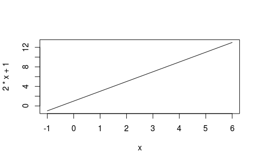
(execute abline(h = 0, v = 0) right after the curve command above if you wish to also see the axes x=0 and y=0)
Take a look at the 01_linear.R script for examples of other linear functions. Notice how the slope a and intercept b affect a shape of a linear function.
A constant function has the form
\[ y = b \]
You may use the following approach to plot a constant function in R:
constFun <- function(x) rep(3, length(x))
curve(constFun, -1, 6)
Absolute Value Functions
An absolute value function is
\[ y = \lvert x \rvert \]
or perhaps even
\[ y = a\lvert x - b\rvert + c \]
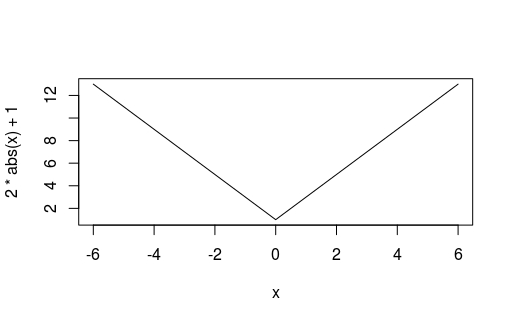
Try plotting the \( y = 2\lvert x \rvert + 1 \) function in R:
curve(2*abs(x) + 1, -6, 6)
Quadratic Functions
A quadratic function has the form
\[ y = ax^2 + bx + c \]
This form is called the standard form. That can be rewriten to a vertex form:
\[ y = a(x + d)^2 + e \]
where \( d = \frac{b}{2a} \) and \( e = -\frac{b^2}{4a} + c \)
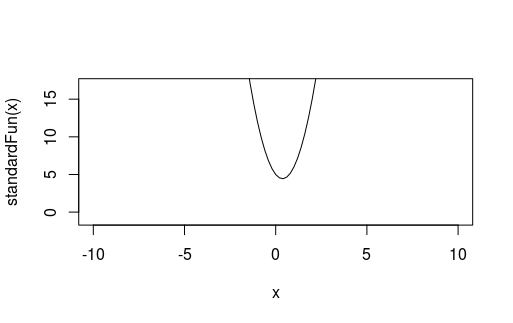
For example, try plotting the function \( y = 4x^2 - 3x + 5 \) (the function is equivalent to \( y = 4(x - \frac{3}{8})^2 - \frac{9}{16} + 5 \) )
standardFun <- function(x) 4*(x^2) - 3*x + 5
curve(standardFun, -10, 10, ylim = c(-1, 17))
Linear Rational Functions
Linear rational functions hava the form
\[ y = \frac{ax + b}{cx + d} \]
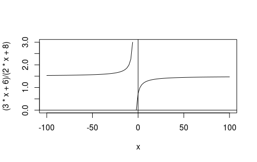
Try plotting the function \( y = \frac{3x + 6}{2x + 8} \)
curve((3*x + 6)/(2*x + 8), -100, 100)
abline(h = 0, v = 0)
Functions with Rational Exponents
Functions with rational exponents have the form
\[ y = x^\frac{a}{b} \]
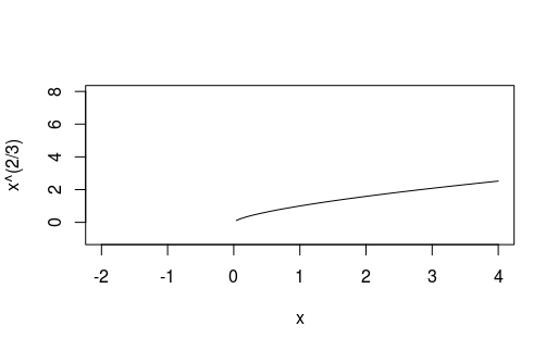
Try plotting a function \( y = x^\frac{2}{3} \)
curve(x^(2/3), -2, 4, ylim = c(-1, 8))
Exponential and Logarithmic Functions
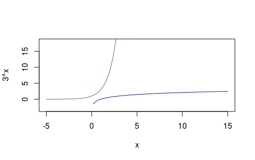
An exponential function has the form \[ y = a^x \]
while a logarithmic function has the form
\[ y = log_ax \]
Try plotting \( y = 3^x \) and \( y = log_3x \)
curve(3^x, -5, 15, ylim = c(-3, 18), col="tan4")
curve(log(x, 3), -5, 15, add = TRUE, col="blue1")
Trigonometric Functions
Trigonometric functions are:
\[ y = sin(x) \] \[ y = cos(x) \] \[ y = tg(x) \] \[ y = cotg(x) \]
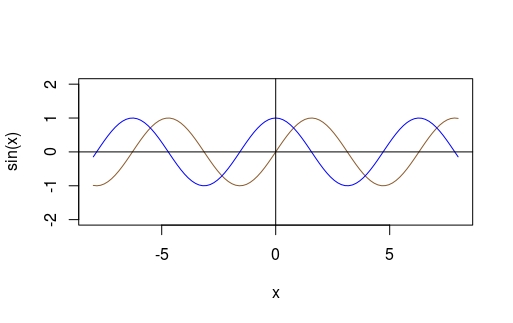
Compare \( y = sin(x) \) with \( y = cos(x) \) in the same plot:
curve(sin(x), -8, 8, col = "tan4", ylim = c(-2, 2))
curve(cos(x), -8, 8, add = TRUE, col = "blue1")
abline(h = 0, v = 0)
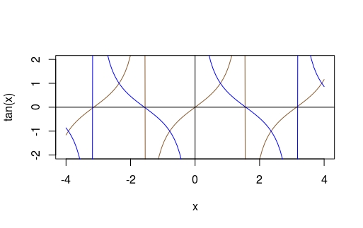
Similarly, compare \( y = tg(x) \) with \( y = cotg(x) \)
curve(tan(x), -4, 4, col = "tan4", ylim = c(-2, 2))
curve(1/tan(x), -4, 4, add = TRUE, col = "blue1")
abline(h = 0, v = 0)