Statistics in R: Binomial Distribution
Let’s use the R and RStudio to learn more about the binomial distribution!
- Downloading the Project
- Introduction
- Generating binomial data
- Probability Density
- Cumulative Density
- Quantiles
- Quantile-Quantile Plots
- Further Reading
Downloading the Project
We will be using the ProbabilityDistributions project, which you can download in the form of a ZIP archive ProbabilityDistributions.zip. After you’ve downloaded the archive, proceed by extracting it, go into a newly created ProbabilityDistributions folder and double-click on the ProbabilityDistributions.Rproj icon. This opens up the ProbabilityDistributions project in the RStudio.
Introduction
This entire paragraph was taken over from the Introduction to Statistical Thought (written by Michael Lavine; published on June 24, 2010).
Statisticians often have to consider observations of the following type:
- A repeatable event results in either a success or a failure.
- Many repetitions are observed
- Successes and failures are counted
- The number of successes helps us learn about the probability of success.
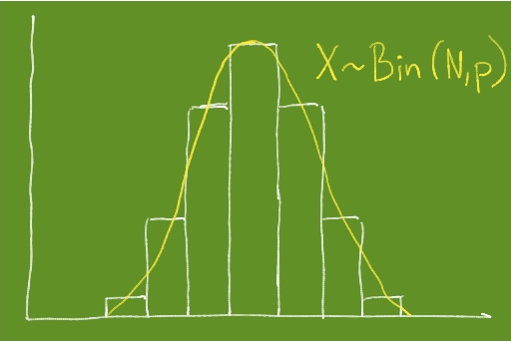
Because binomial experiments are so prevalent there is specialized language to describe them. Each repetition is called a trial; the number of trials is usually denoted N; the unknown probability of success is usually denoted either p or θ; the number of successes is usually denoted X. We write _X ∼ Bin(N, p) _. The symbol “∼” is read is distributed as; we would say “X is distributed as Binomial N p” or “X has the Binomial N, p distribution”.
Some important assumptions about binomial experiments are that N is fixed in advance, θ is the same for every trial, and the outcome of any trial does not influence the outcome of any other trial.
Generating binomial data
Let’s create a function summarize.binomial.observations, which takes the following parameters:
- trials - a number of trials (N)
- theta - a probability of success (θ)
- observations - a number of observations to be made
library(tidyverse)

summarize.binomial.observations <- function(trials, theta, observations) {
  sample.space <- c(1,0)
  results <- 1:observations %>%
  map_int(function(x)
    as.integer(
      sum(
        sample(sample.space, size = trials, replace = TRUE, prob = c(theta, 1 - theta))
      )
    )
  )
  return(results)
}
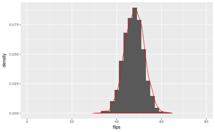
Now we can use the function to generate 3000 observations of X ∼ Bin(80, 0.6):
summary <- summarize.binomial.observations(80, 0.6, 3000)
resulting.df <- data.frame(flips <- summary) # ggplot only works with data frames
names(resulting.df) <- c("flips")
#binPDF <- data.frame(x<-1:80, y<-dbinom(1:80, size=80, prob = 0.6))
#names(binPDF) <- c("flips", "prob")

ggplot(resulting.df) +
  geom_histogram(breaks=seq(1, 80, 2), aes(x=flips, y=..density..), position="identity") +
  geom_density(aes(x=flips, y = ..density..), colour="red")
It turns out that R already contains a function which produces the same data as summarize.binomial.observations. The function is called rbinom and it repeatedly performs a random draw from a binomial distribution.
drawsV1 <- summarize.binomial.observations(80, 0.6, 3000)
drawsV2 <- rbinom(3000, 80, 0.6)
mean(drawsV1)
mean(drawsV2)
length(drawsV1)
length(drawsV2)
produces:
[1] 48.01467
[1] 48.052
[1] 3000
[1] 3000
Probability Density
The probability of observing exactly 5 heads out of 10 flips can be estimated as
mean(rbinom(1000, 10, .5) == 5)
result:
[1] 0.232
There is a special function in R which calculates the probability density - it is called dbinom:
dbinom(5, 10, .5)
yields:
[1] 0.2460938
Cumulative Density
The probability of observing exactly at most 4 heads out of 10 flips can be estimated as
mean(rbinom(1000, 10, .5) <= 4)
result:
[1] 0.392
There is a special function in R which calculates the cumulative density - it is called pbinom:
pbinom(4, 10, .5)
output:
[1] 0.3769531
Quantiles
Quantile works as an inverse of the cumulative density function, as illustrated below:
qbinom(pbinom(4, 10, .5), 10, .5)
[1] 4
Visit Basic Probability Distributions in R for more information.
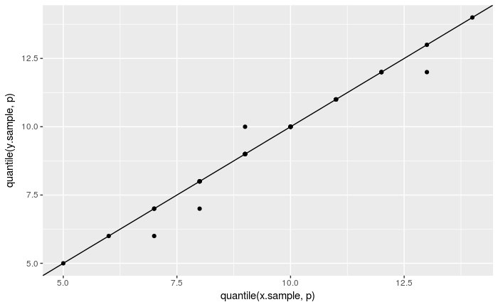
Quantile-Quantile Plots
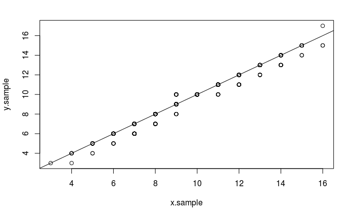
As described in the Q-Q Plot Tutorial, The quantile-quantile (q-q) plot is a graphical technique for determining if two data sets come from populations with a common distribution.
The following code compares observations stored in x.sample with those in y.sample:
x.sample <- rbinom(1000, 19, .5)
y.sample <- rbinom(1000, 19, .5)
qqplot(x.sample, y.sample)
abline(0,1)
The same test using ggplot2:
nq <- 31
p <- (1 : nq) / nq - 0.5 / nq
ggplot() + geom_point(aes(x = quantile(x.sample, p), y = quantile(y.sample, p))) +
  geom_abline(intercept = 0, slope = 1)
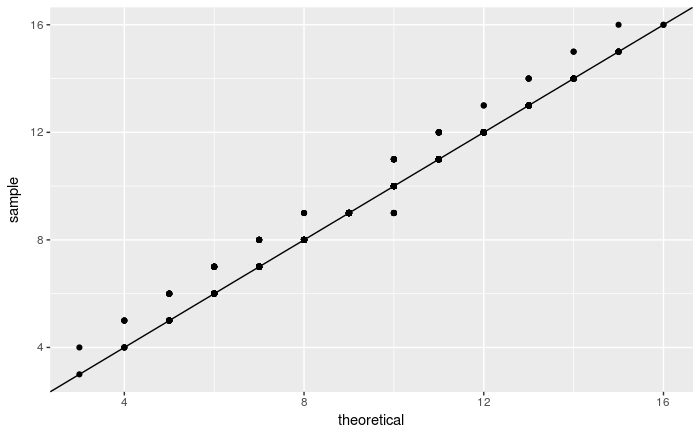
Do the following to compare the x.sample with a binomial distribution Bin(19, 0.5):
xdf <-data.frame(x = x.sample)
ggplot(xdf, aes(sample = x)) +
  stat_qq(distribution = stats::qbinom, dparams = list(size = 19, prob=0.5)) +
  geom_abline(intercept = 0, slope = 1)