Statistics in R: Poisson Distribution
Let’s use the R and RStudio to learn more about the Poisson distribution!
- Downloading the Project
- Introduction
- Generating Poisson data
- Probability Density
- Cumulative Density
- Quantiles
- Quantile-Quantile Plots
- Further Reading
Downloading the Project
We will be using the ProbabilityDistributions project, which you can download in the form of a ZIP archive ProbabilityDistributions.zip. After you’ve downloaded the archive, proceed by extracting it, go into a newly created ProbabilityDistributions folder and double-click on the ProbabilityDistributions.Rproj icon. This opens up the ProbabilityDistributions project in the RStudio.
Introduction
This entire paragraph was taken over from the Introduction to Statistical Thought (written by Michael Lavine; published on June 24, 2010).
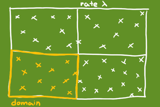
Poisson observations occur in the following situation:
- There is a domain of study, usually a block of space or time.
- Events arise seemingly at random in the domain.
- There is an underlying rate at which events arise.
Such observations are called Poisson after the 19th century French mathematician Siméon- Denis Poisson. The number of events in the domain of study helps us learn about the rate.
The rate at which events occur is often called λ; the number of events that occur in the domain of study is often called X; we write X ∼ Poi(λ). Important assumptions about Poisson observations are that two events cannot occur at exactly the same location in space or time, that the occurence of an event at location \(l_1\) does not influence whether an event occurs at any other location \(l_2\), and the rate at which events arise does not vary over the domain of study.
Generating Poisson data
In the following simulation of a Poisson distribution, we are going to uniformly pick 200 points from a square of 5000x5000 points. The square can be divided into four quadrants, each having 2500x2500 points. Each of the four quadrants can be thought of as a separate domain of study and the rate with which points are picked from a given domain is \(λ = \cfrac{200}{4} = 50\)
The probability of picking exactly X points from the first quadrant follows a Poisson distribution X ~ Poi(50).
Let’s create a function summarize.poisson.observations, which takes the following parameters:
- lambda - a rate with which events occur in a given domain
- observations - a number of observations to be made
library(tidyverse)

summarize.poisson.observations <- function(lambda, observations) {
  results <- results <- 1:observations %>%
    map_int(function(x)
      as.integer(
        count(
          filter(data.frame(x = sample(5000, size=4*lambda, replace=FALSE), y = sample(5000, size=4*lambda, replace=FALSE)),
                 x <= 2500,
                 y <= 2500)
        )
      )
    )
  return(results)
}
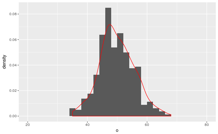
Now we can use the function to generate 400 observations of X ∼ Poi(50):
summary <- summarize.poisson.observations(50, 400)
resulting.df <- data.frame(o <- summary) # ggplot only works with data frames
names(resulting.df) <- c("o")
#binPDF <- data.frame(x<-1:80, y<-dbinom(1:80, size=80, prob = 0.6))
#names(binPDF) <- c("flips", "prob")

ggplot(resulting.df) +
  geom_histogram(breaks=seq(20, 80, 2), aes(x=o, y=..density..), position="identity") +
  geom_density(aes(x=o, y = ..density..), colour="red") # + geom_line(data=binPDF, aes(flips, prob), colour="blue")
It turns out that R already contains a function which produces the same data as summarize.poisson.observations. The function is called rpois and it repeatedly performs a random draw from a Poisson distribution.
drawsV1 <- summarize.poisson.observations(50, 400)
drawsV2 <- rpois(400, 50)
mean(drawsV1)
mean(drawsV2)
length(drawsV1)
length(drawsV2)
produces:
[1] 49.95
[1] 50.175
[1] 400
[1] 400
Probability Density
The probability of observing exactly 49 events in a given domain, given the rate is 50, can be estimated as
mean(rpois(400, 50) == 49)
result:
[1] 0.05
There is a special function in R which calculates the probability density - it is called dpois:
dpois(49, 50)
yields:
[1] 0.05632501
Cumulative Density
The probability of observing at most 45 events in a given domain, given the rate is 50, can be estimated as
mean(rpois(400, 50) <= 45)
result:
[1] 0.2975
There is a special function in R which calculates the cumulative density - it is called ppois:
ppois(45, 50)
output:
[1] 0.2668665
Quantiles
Quantile works as an inverse of the cumulative density function, as illustrated below:
qpois(ppois(45, 50), 50)
[1] 45
Visit Basic Probability Distributions in R for more information.
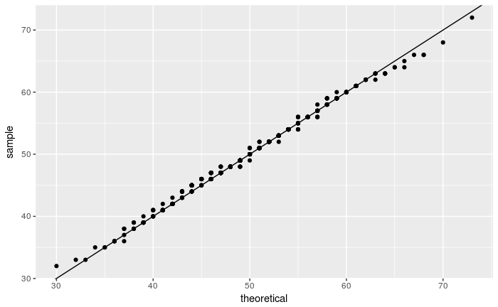
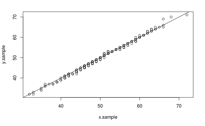
Quantile-Quantile Plots
As described in the Q-Q Plot Tutorial, The quantile-quantile (q-q) plot is a graphical technique for determining if two data sets come from populations with a common distribution.
The following code compares observations stored in x.sample with those in y.sample:
x.sample <- rpois(400, 50)
y.sample <- rpois(400, 50)
qqplot(x.sample, y.sample)
abline(0,1)
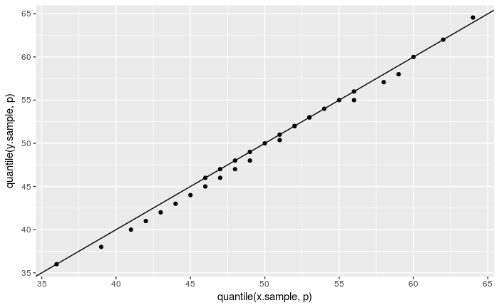
The same test using ggplot2:
nq <- 31
p <- (1 : nq) / nq - 0.5 / nq
ggplot() + geom_point(aes(x = quantile(x.sample, p), y = quantile(y.sample, p))) +
  geom_abline(intercept = 0, slope = 1)
Do the following to compare the x.sample with a Poisson distribution Poi(50):
xdf <-data.frame(x = x.sample)
ggplot(xdf, aes(sample = x)) +
  stat_qq(distribution = stats::qpois, dparams = list(lambda=50)) +
  geom_abline(intercept = 0, slope = 1)